Benchmarking Report¶

In this report we compare the performance of odc-stac (GitHub, Docs) and stacktac (GitHub, Docs) libraries when loading Sentinel-2 COG (Cloud Optimized GeoTIFF) data from Azure blob storage. We analyse relative performance of the two libraries in the two common data access scenarios and measure the effect of Dask chunk-size choice on observed performance.

Experiment Setup¶

Experiment was conducted in the Planetary Computer Pangeo Notebook environment, using a single-node Dask cluster with 4 cores and 32 GiB RAM.

We load three bands (red, green and blue) in the native projection and resolution of the data (10m, UTM). We consider two scenarios: deep (temporal processing) and wide (building mosaic for visualisation).

deep temporal data: 2 months worth of data for a single Sentinel-2 granule

3 bands, 13 time slices, 10,980x10,980 pixels each, 8.76 GiB
repeated with various chunk sizes

STAC API query

{
   "collections": ["sentinel-2-l2a"],
   "datetime": "2020-06/2020-07",
   "query": {
       "s2:mgrs_tile": {"eq": "35MNM"},
       "s2:nodata_pixel_percentage": {"lt": 10}
   }
}

STAC Features Deep

wide area data: 1 day worth of data across 9 Sentinel-2 granules
- 3 bands, 1 time slice, 10,980x90,978 pixels each, 5.58 GiB
- repeated with various chunk sizes
- repeated with different output resolutions (aligned to internal overview resolutions of the data)
- STAC API query
```
{
   "collections": ["sentinel-2-l2a"],
   "datetime": "2020-06-06",
   "bbox": [27.345815, -14.98724, 27.565542, -7.710992]
}
```
- STAC Features Wide

To control for variability in data access performance, we run each benchmark several times and pick the fastest run for comparison. Most configurations were processed five times, with some slower ones being repeated three times. We have observed low variability of execution times for the slower ones.

A rotated thumbnail of the wide area scenario is displayed below, the image is actually tall and narrow - to save space we display it rotated counter clockwise.

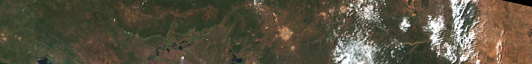
The deep scenario was taken from the same region, but using only one granule (35MNM, left side of the image above).

Deep Scenario Results¶

To investigate the impact of the configuration choices we consider several chunking sizes. When loading deep scenario data, we find that for both odc-stac and stackstac, chunk size of 2048 pixels produces the best result. When using optimal configuration, stackstac achieves a peak throughput of 121.8 output megapixels per second (Mpix/s), which is about 15% higher than odc-stac which peaks at 105 Mpix/s.

Both libraries use GDAL via rasterio to read the data, but stackstac configures GDAL internal caching to optimize the re-use of the image metadata. This has significant positive impact on performance. Essentially, caching is only enabled when reading the image headers, so they don't get ejected by the compressed pixel data, because the compressed data is read without caching. This is especially helpful when using multiple threads in Dask workers.

Wide Scenario Results¶

When loading a large mosaic however,odc-stac has a significant advantage over stackstac. For odc-stac optimal chunk size remains the same as for the deep scenario: 2048 pixels. For stackstac, performance slowly improves with the larger chunk sizes. The best performance for stackstac was achieved using the largest chunk size we tried: 7168 pixels. Throughput achieved by odc-stac is almost 2.5 times higher than stackstac: 74.7 vs 30.1 Mpix/s.

The approach taken by stackstac for loading mosaics is roughly as following:

Create one pixel plane for each STAC item being loaded, and stack them into one Dask Array (same as a temporal load)

Use Xarray and Dask to merge those layers

xx = stackstac.stack(items, ...)
mosaic = xx.groupby("time").map(stackstac.mosaic)

This means that the computational complexity of the wide scenario grows with the number of STAC items being loaded and not just with the number of output pixels being produced. A single large area STAC Item will load significantly faster than the same area partitioned into many STAC Items.

This approach to data loading results in a very large Dask graph with a large number of "no-op" chunks. While stackstac includes optimizations for chunks that are "empty", those still need to be processed by the Dask scheduler, resulting in a significant processing overhead.

Approach taken by odc-stac avoids this problem:

For each output Dask chunk, figure out what data overlaps with this chunk at the Dask graph construction time
For chunks that have no data, generate an "empty" task (returns array filled with nodata values)
For chunks that have only one data source, generate a "simple load" task
For chunks with multiple data sources, generate a "fused load" task, i.e. load data from multiple sources and, for each output pixel, pick one valid observation in the deterministic fashion (first observed non-empty pixel is used for the output).

As a result, Dask graph produced by odc-stac is much smaller than the graph produced by stackstac in this scenario. Which results in a much faster submission and processing by the Dask scheduler. The table below lists the Submit time in seconds, as observed for the fastest run across the chunk sizes.

chunk	512	1024	2048	3072	4096	5120	6144	7168
odc-stac	3.881	0.927	0.272	0.116	0.084	0.238	0.034	0.029
stackstac	33.366	7.950	1.967	0.778	0.484	0.426	0.156	0.136

Slow submit times are especially inconvenient in interactive data analysis workflows.

Comparing Wide vs Deep¶

Both odc-stac and stackstac achieve lower throughput when constructing mosaics vs loading a column of pixel data, but the penalty is significantly higher for stackstac.

Sentinel-2 granules have some duplicated pixels. As a result, one needs to load several input pixels for some of the output pixels, and then combine them somehow into one (usually pick one out of the several valid candidates). In the wide scenario, we need to load about 1.08 input pixels for every output pixel, while for deep scenario input to output ratio is exactly 1. More work needs to be done per output pixel for the wide scenario, and so one should expect somewhat lower throughput.

For odc-stac, throughput for the wide scenario is about 30% lower than for the deep (74.7 vs 105 Mpix/s). From the pixel overlap cost alone, one would expect an 8% higher work requirement on the read side. The other 22% could be explained by the pixel-fusing computational requirements.

For stackstac, building mosaics is significantly more expensive computationally than reading temporal columns of data (30.1 vs 121.8 Mpix/s peak throughput, around 4 times slower per output pixel in wide scenario).

Generating Overview Image¶

Loading data at significantly reduced resolutions is a common scenario. And is especially useful in the exploratory stages of the data analysis, which tend to be interactive and thus benefit from faster load times.

The cloud-optimized imagery includes low-resolution overviews, and therefore can be read much faster at lower resolutions. For every doubling of the output pixel size in ground units, one needs to load four times fewer input pixels for the same geographic area.

Table: Performance across resolutions¶

	elapsed	throughput_mps
10	40.1	165.9	74.7	18.1
20	9.9	77.1	75.5	9.7
40	6.3	56.3	29.6	3.3
80	2.3	29.3	20.6	1.6

For odc-stac, reading imagery at 20m pixels is 4 times faster than reading at the native 10m. Throughput per output pixel remains the same but there are four times fewer pixels to read. At the higher zoom out scales throughput starts to drop off, but load times are still getting quite a bit faster the further you zoom out.

For stackstac, lower resolution reads do result in faster completion time, but throughput per output pixel drops off much quicker than for odc-stac.

When zooming out to 1/8 image side size (1/64 in the number of pixels), odc-stac is more than 10 times quicker than stackstac (2.3 vs 29.3 seconds).

	chunk	512	1024	2048	3072	4096	5120	6144	7168
method	scenario
odc-stac	wide	154.2	65.4	40.1	43.9	55.2	54.6	55.1	55.0
stackstac	wide	470.1	236.3	165.9	127.4	117.8	111.5	102.8	99.6
odc-stac	deep	183.9	77.0	44.8	45.3	60.0	69.6	68.9	69.1
stackstac	deep	212.1	76.6	38.6	43.4	56.4	66.4	68.6	69.4

	chunk	512	1024	2048	3072	4096	5120	6144	7168
method	scenario
odc-stac	wide	19.4	45.8	74.7	68.3	54.3	54.8	54.4	54.5
stackstac	wide	6.4	12.7	18.1	23.5	25.4	26.9	29.2	30.1
odc-stac	deep	25.6	61.1	105.0	103.8	78.4	67.6	68.2	68.0
stackstac	deep	22.2	61.4	121.8	108.3	83.3	70.8	68.5	67.8

Benchmarking Report¶

Experiment Setup¶

Deep Scenario Results¶

Wide Scenario Results¶

Comparing Wide vs Deep¶

Generating Overview Image¶

Table: Performance across resolutions¶

Acknowledgements¶

Appendix¶

Results for 10m data load¶

Table: Elapsed seconds¶

Table: Submit seconds¶

Table: Throughput (Mpix/s)¶

Results for Different Resolutions¶

Table: Elapsed seconds, different resolutions¶

Table: Submit seconds, different resolutions¶

Table: Throughput (Mpix/s), different resolutions¶

	resolution	10	20	40	80
method	chunk
odc-stac	512	3.881	0.865	0.162	0.047
	1024	0.927	0.161	0.047	0.020
	2048	0.272	0.047	0.020	0.010
stackstac	512	33.366	8.782	2.281	0.352
	1024	7.950	2.272	0.504	0.438
	2048	1.967	0.660	0.434	0.039